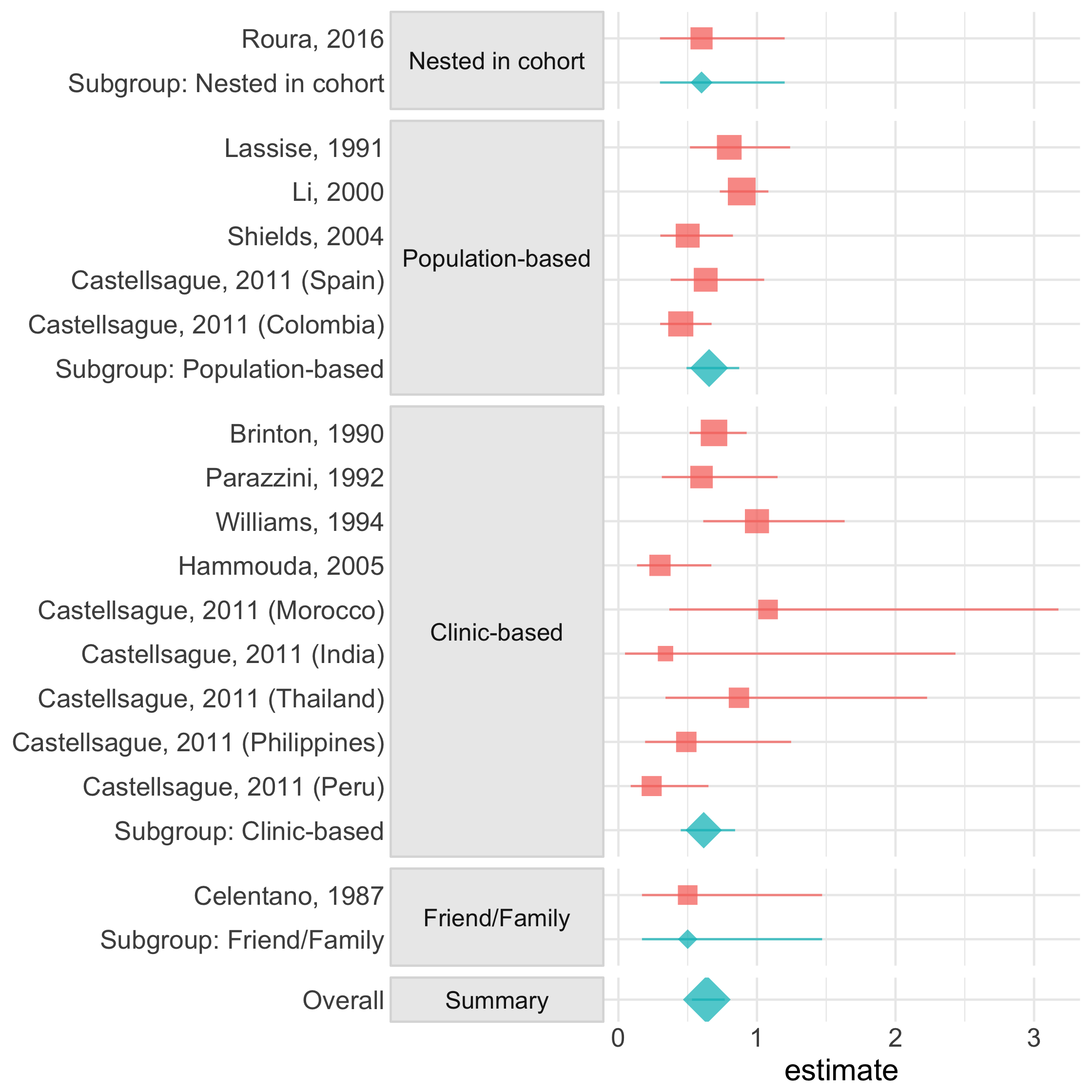
forest_plot()
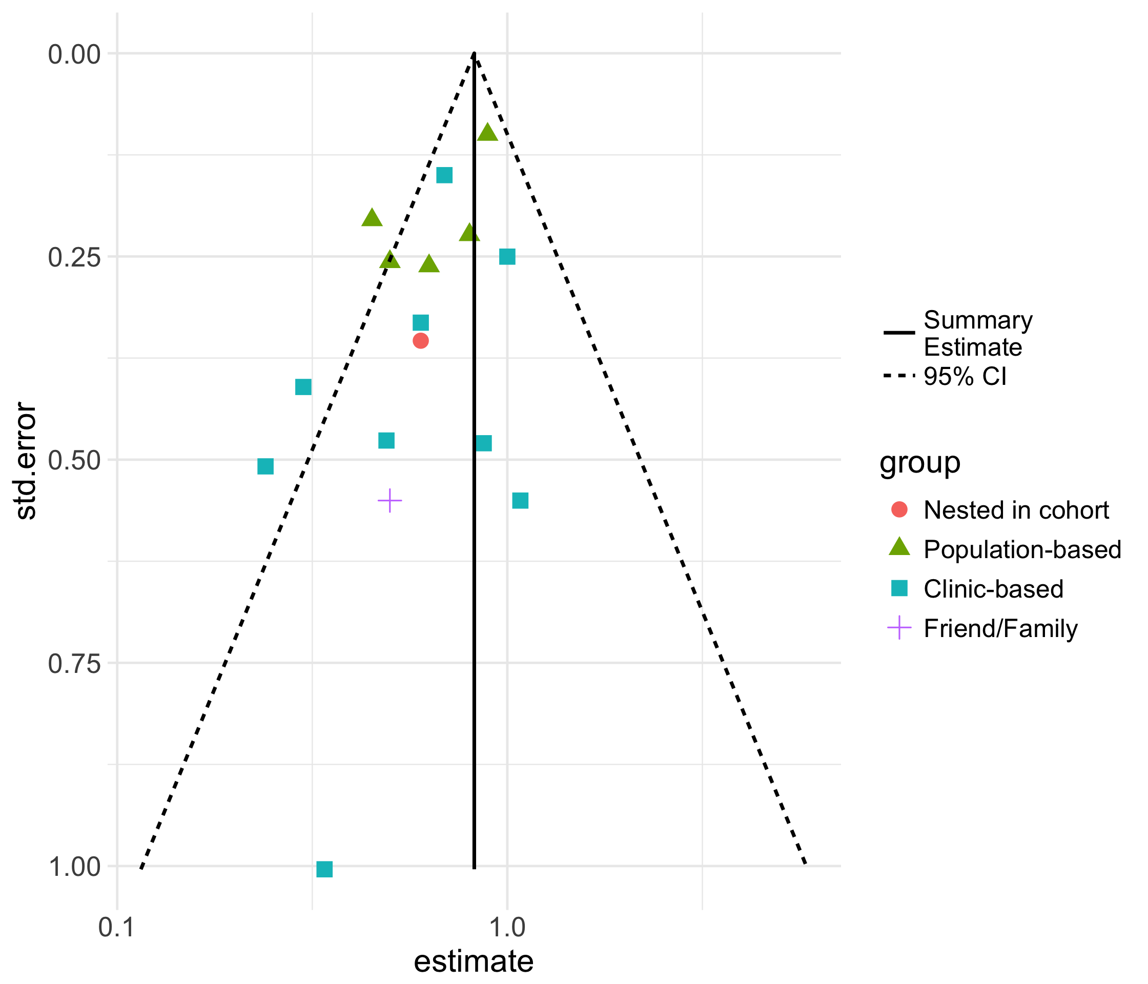
funnel_plot()
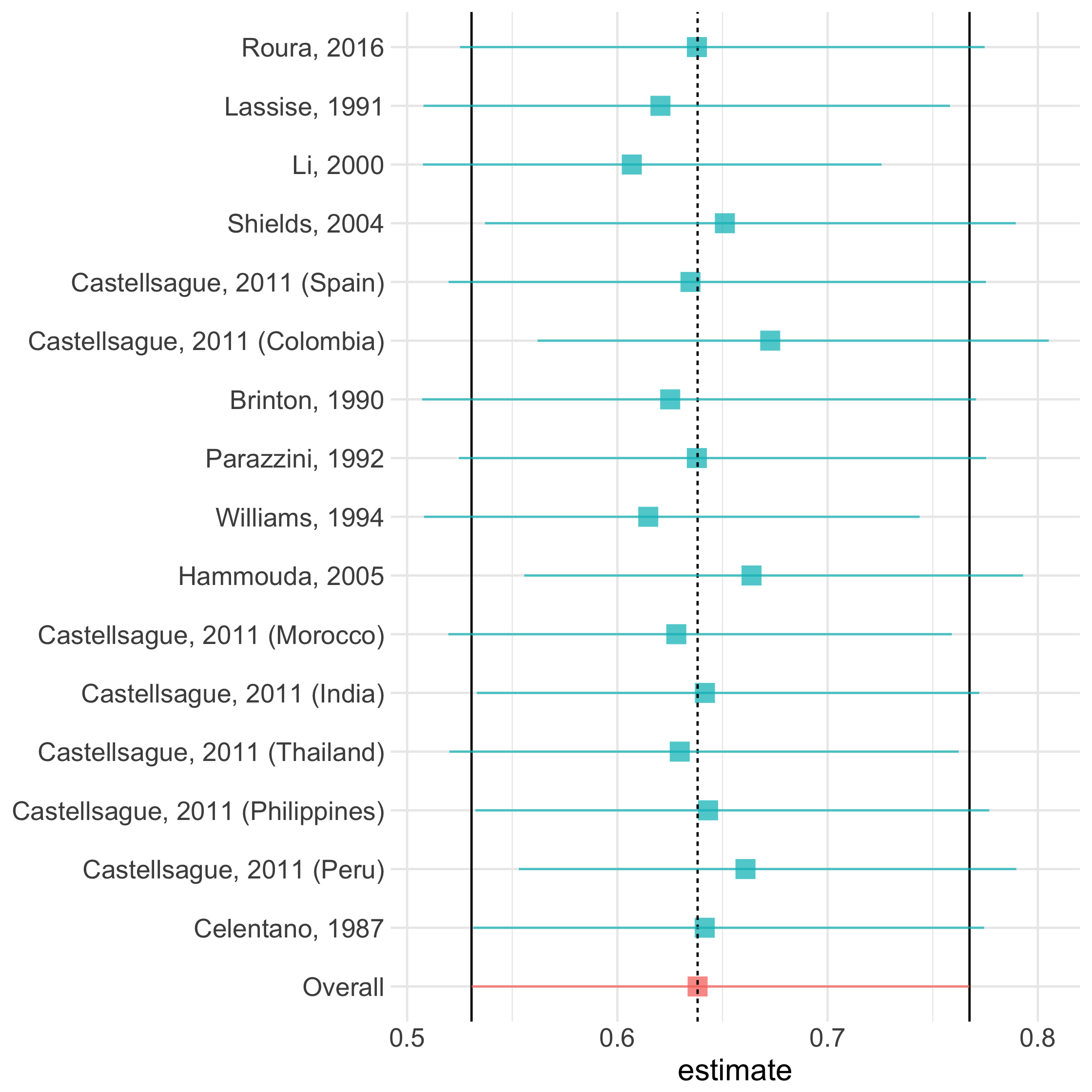
influence_plot()
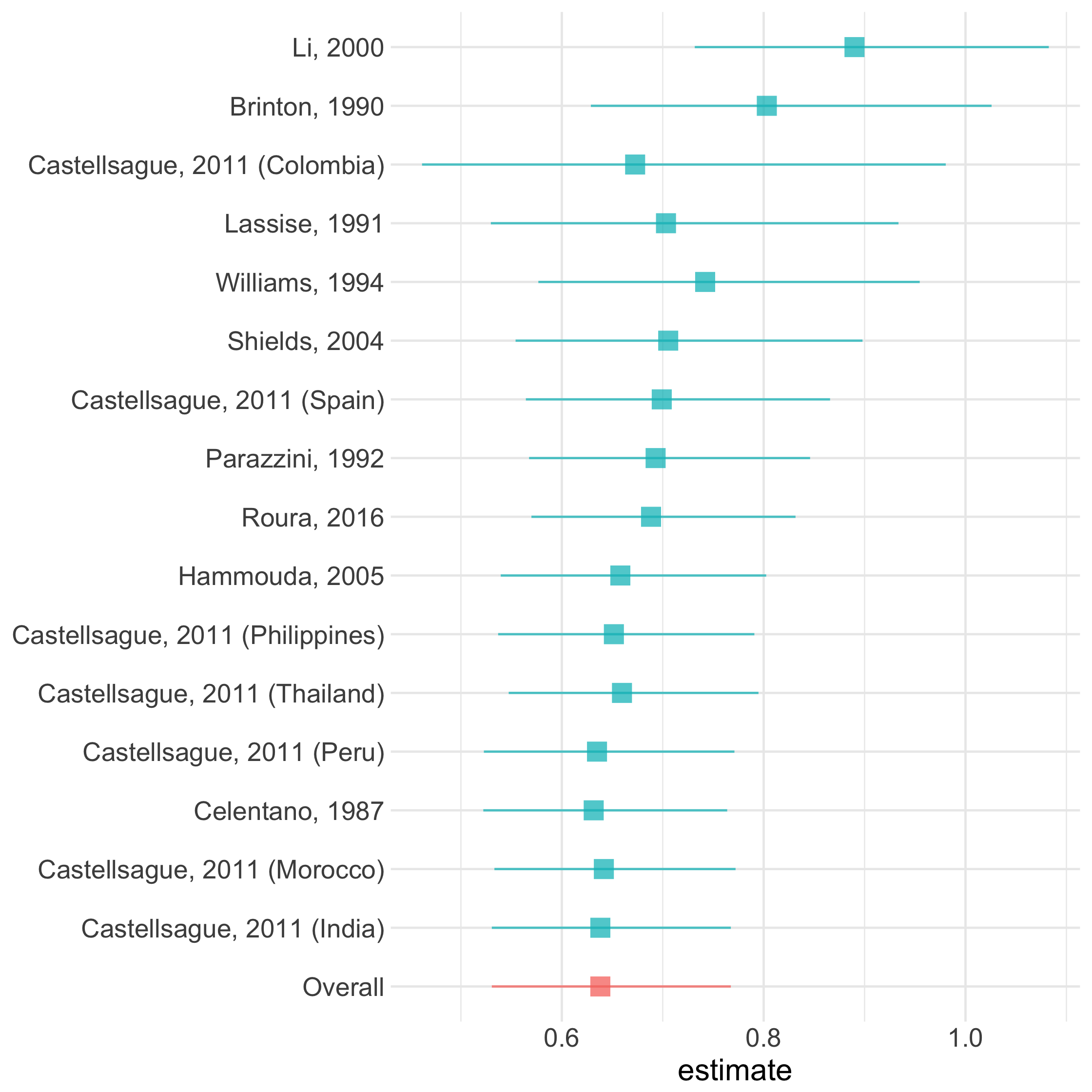
cumulative_plot()
library(ggplot2)p <- ggplot(iud_cxca, aes(case_num + control_num, lnes, color = group))p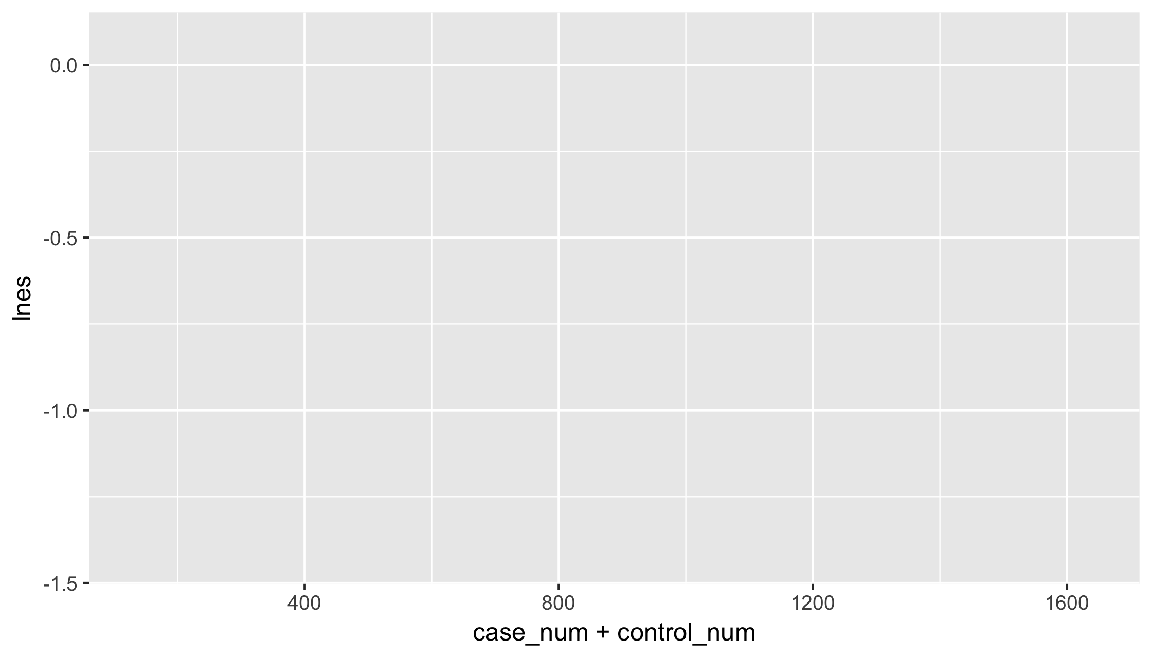
library(ggplot2)p <- p + geom_point()p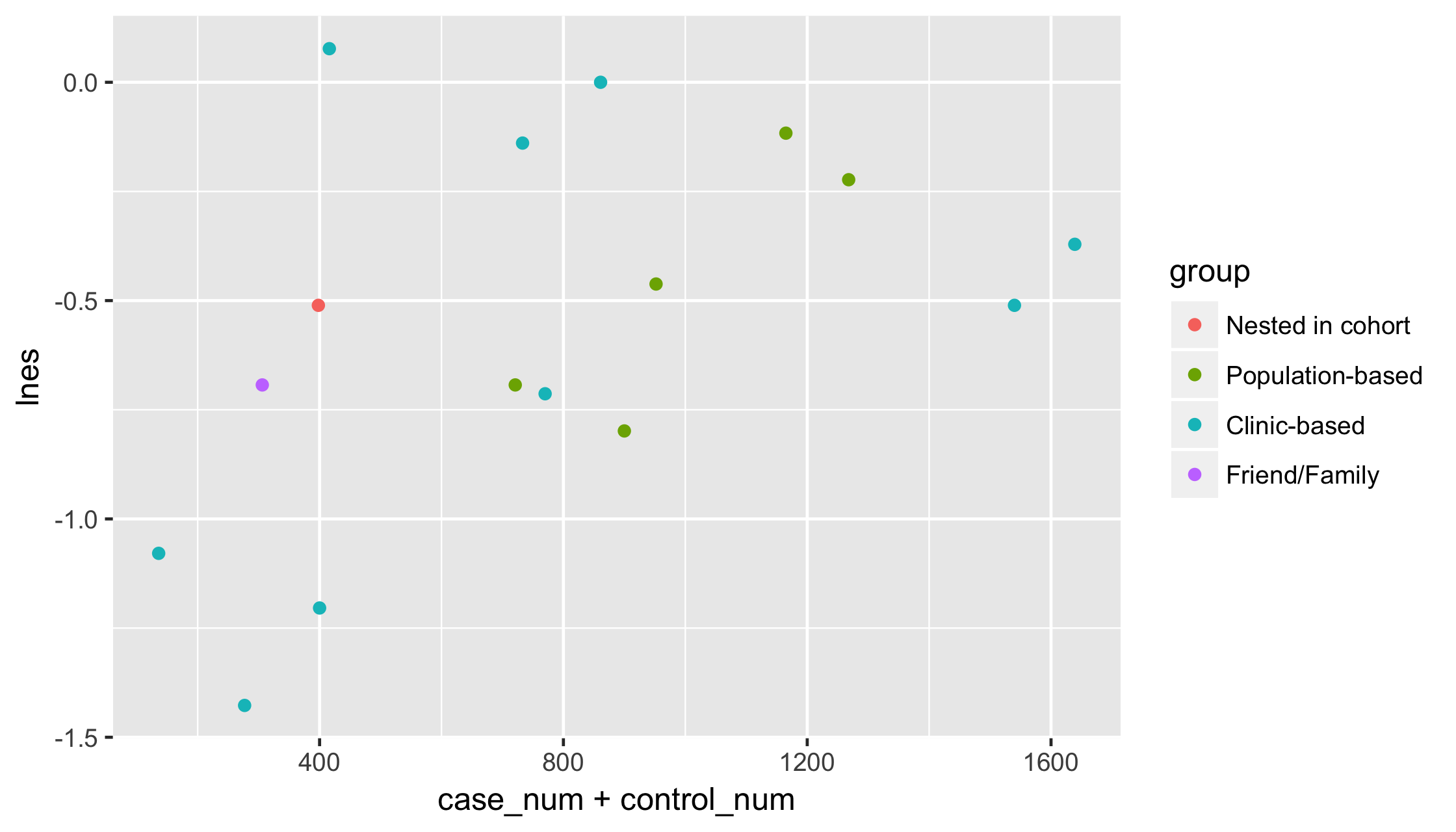
p <- p + geom_smooth(method = "lm", se = FALSE)p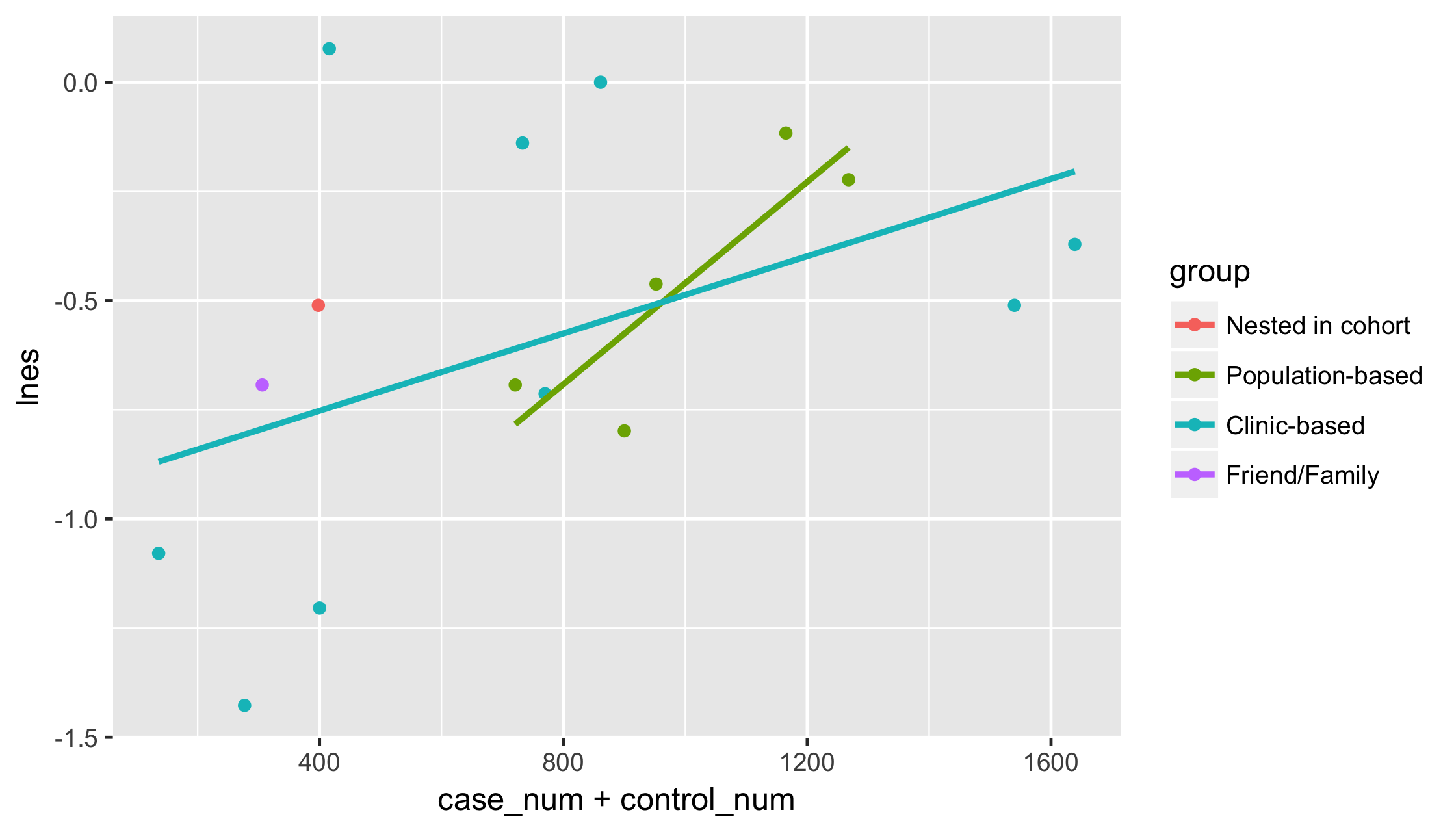
p + labs(title = "The Effect of Sample Size on Estimate", x = "Sample Size", y = "ln(Odds Ratio)") + scale_color_discrete(name = "Study Design") + theme_minimal() + theme(text = element_text(size = 16))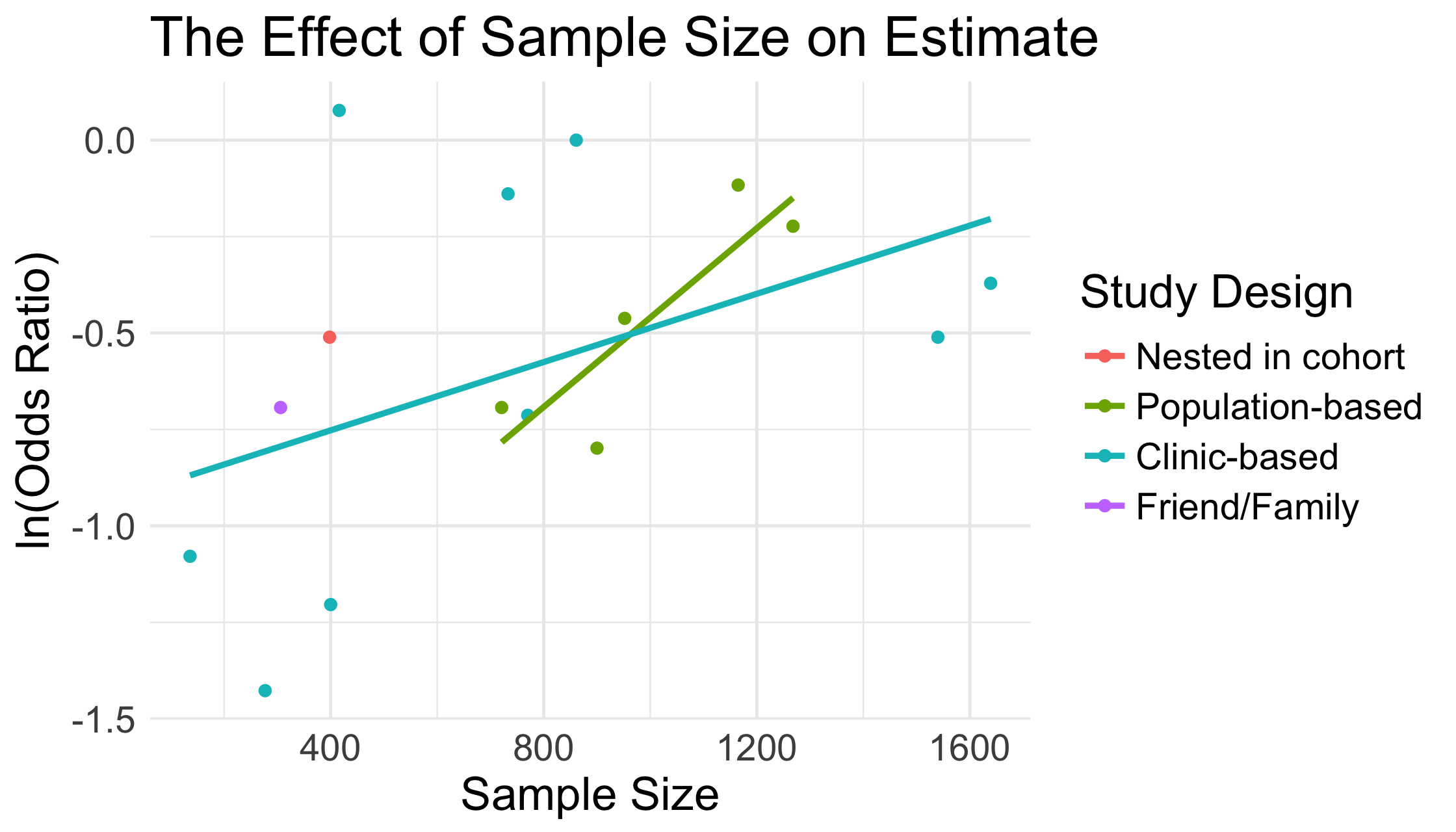
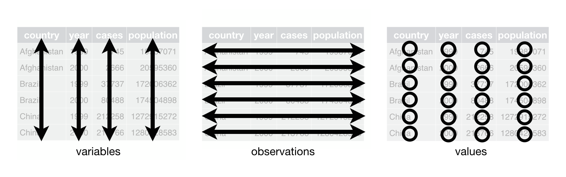
Tidy Data is Easier to Plot
Tidy Data is Easier to Plot
Each column is a single variable
Tidy Data is Easier to Plot
Each column is a single variable
Each row is a single observation
Tidy Data is Easier to Plot
Each column is a single variable
Each row is a single observation
Each cell is a value
Our Tidy Tools
%>%
mutate()
arrange()
group_by()
tidy()

Our Tidy Tools
%>%: passes the results of one function to the next
mutate()
arrange()
group_by()
tidy()
Our Tidy Tools
%>%
mutate(): changes or creates a new variable
arrange()
group_by()
tidy()
Our Tidy Tools
%>%
mutate()
arrange(): sorts a data set by a variable
group_by()
tidy()
Our Tidy Tools
%>%
mutate()
arrange()
group_by(): groups a data set by a variable
tidy()
Our Tidy Tools
%>%
mutate()
arrange()
group_by()
tidy(): tidies statistical results
patchwork: Compose ggplots
![]()
patchwork: Compose ggplots
Join ggplots quickly and accurately
![]()
patchwork: Compose ggplots
Join ggplots quickly and accurately
library(patchwork)forest_plot() + text_table()![]()

github.com/malcolmbarrett/tidymeta
github.com/malcolmbarrett/ma_viz_workshop
Slides created via the R package xaringan.